Simulation-based Dynamic Shop Floor Scheduling For a Flexible Manufacturing System in the Industry 4.0 Environment

by Wenhe Yang Soemon Takakuwa (Chuo University)

As presented at the 2017 Winter Simulation Conference

The Industry 4.0 environment enables direct communication between the manufacturer’s shop floor and a customer. Thus, the manufacturer is able to respond to the customers’ requests more quickly, meaning that manufacturers must now more tightly control the shop floor planning and scheduling. Here we present a simulation-based scheduling model for Flexible Manufacturing System dynamic shop-floor control. The customer’s order and the processing sequence table of the products are imported into the simulation model. Experiments are implemented for the case wherein the system encounters unexpected conditions. The proposed approach represents a potential tool for manufacturers to make decisions in the real time by further connecting to the Enterprise Resource Planning and Manufacturing Execution System.

Introduction

In an Industry 4.0 environment, cyber-physical systems communicate with each other and with human participants in real time via the Internet of Things (IoT). This enables direct communication between the manufacturer’s shop floor and a customer, and thus, mass customization will be adopted as a production system (Takakuwa 2016). Process planning and scheduling problems in the manufacturing system that assigns jobs and materials to machines and decides job processing sequences severely affect the system performance. Under the Industry 4.0 environment, the increasing customization of products requires that these systems handle higher numbers of product variants as well as smaller lot sizes, and therefore manufacturing systems are becoming more and more complex to cope with these uncertain situations (Kück et al. 2016).

The Flexible Manufacturing System (FMS) is an integrated system of manufacturing machine modules and material-handling equipment under a computer system’s control and enables automatic random processing of palletized parts (ElMaraghy 2005). The FMS is highly automated and complex, and each machine can process at most one job at a given time. However, arranging which job is assigned to which machine and maintaining control of the shop floor in a job-shop system is more difficult than in a flow-shop system due to the dynamic variation. Therefore, the simulation method is a well-proven approach to design and analyze the FMS.

Traditional planning and scheduling research focus on how to give a determined schedule to the system. However, when manufacturing systems encounter unexpected conditions, such as machine breakdown and rush orders, the predetermined schedule may no longer be the optimal one or may become inoperative due to these unexpected disruptions (Zhang and Wong 2017). Furthermore, as processing time variability increases, decisions can be made by dispatching rules or other heuristics, rather than generating a full schedule prior to the actual production (Vieira, Herrmann, and Lin 2003).

The state of the art in real-time scheduling in manufacturing system with machining and assembly operations, that including the studies focused on job-shop and flow-shop, has been reviewed by Khodke and Bhongade (2013). According to their summaries, event driven and with affected operation rescheduling methodology needs further investigations, because most appropriate framework could be consideration of sufficient number of jobs handled with predictive–reactive strategy. Additionally, few studies have considered the transfer time between the machines or real-time simulations.

In this study, a simulation-based scheduling model for FMS shop-floor control is constructed and used to examine the case that system encounters unexpected conditions. This paper is structured as follows: Section 2 presents a brief description of the FMS factory model as well as the shop flow control under the Industry 4.0 environment. In Section 3, the detailed modeling method based on a simulation scheduler is introduced. Then, scheduling applications are performed in both the usual state case and the new order case in Section 4. Finally, conclusions are presented in Section 5.

GENERAL DESCRIPTIONS

2.1 The FMS Factory Model

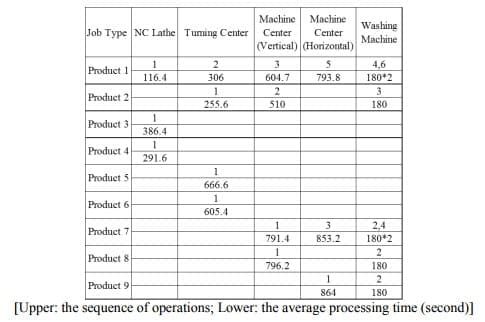
The system considered in this study is an FMS factory model (Takakuwa 1997) located at Chiba Prefecture, Japan. The FMS comprises four NC machine tools, (one NC lathe, one turning center, two types of machine centers (vertical and horizontal)), one washing machine, two AGVs, and one AS/RS with an industrial robot. The facility layout and the distance scale (unit: cm) of the FMS is shown in Figure 1. Workparts are transferred by the AGV and set up by the robot inside the AS/RS. Then, each workpart is loaded by the industrial robot associated with each machine tool prior to machining, then unloaded and after machining. The operation sequences and the associated historical average processing times (including the robot unloading and loading times) for selected workparts are summarized in Table 1. In addition, each workpart is set up for machining by the industrial robot inside the AS/RS before machining at the vertical (V.) machine center and the horizontal (H.) machine center. The AGV returns to the waiting area while idle.

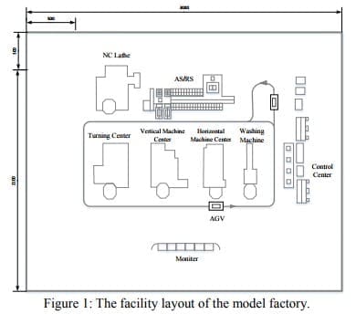
Table 1: The machining sequence and average processing time of the products.

2.2 Shop Floor Control under the Industry 4.0 Environment

The fourth industrial revolution or Industry 4.0 is a collective term representing a number of technologies for automation, data exchange, and supply chain, including manufacturing systems via the Internet of Things (Takakuwa 2016; Wang et al. 2016). Customers’ mass production needs necessitate manufacturer responses to be quicker than ever before.

There are two types of integration in the Factory under the Industry 4.0 environment: vertical integration and horizontal integration. The former is integration from top management through the shop floor inside a factory, i.e., this integration occurs at the company level, the factory level, and the process level, as illustrated in Figure 2. The latter is integration between the suppliers, sales and distribution departments, and customers. In vertical integration, the interaction between the Enterprise Resource Planning (ERP) and Manufacturing Execution System (MES), in conjunction with data from the factory, is important.

Corporations use the ERP to collect, store, manage, and interpret data from various business activities,including procurement, production, distribution, accounting, human resource, sales, and customer services.

The ERP is important because the system monitors real-time data and transaction data in a variety of ways and also monitors shop-floor data and information in the Industry 4.0 environment. The ERP system typically falls short in production scheduling, and ERP solutions have several shortcomings that are widely recognized. For the most part, the ERP system and the day-to-day production remain disconnected. On the other hand, the MES is a control system for the associated shop floor. Manufacturing data are received from machines, equipment monitors, and workers. The MES is integrated with the ERP system.

In order to effectively make real-time decisions that are essential to the manufacturing system, realtime simulation is required. A real-time simulation is a simulated model of a physical system that can simulate processes at the same rate as the actual physical system executes them. the collection of production achievements, planning, instructions sent to the shop floor, and detailed records of performance are to be considered.

Furthermore, Automatic data-capturing systems using RFID or various type of sensors, which could trace and track shop floor data, disturbances and deliver solution adaptive to the real-time shop-floor changes (Khodke and Bhongade 2013).

3 SIMULATION MODEL

Simio Scheduling Tool

The simulation software and the scheduler developed by Simio LCC, is used in this research. Simio is a simulation-modeling framework based on graphical object-oriented programming. The model is realized using multiple modeling paradigms, including event, process, object, system-dynamics, and agentmodeling views (Thiesing and Pegden 2014). Furthermore, Simio is designed to support applications in both system design and scheduling and has several advanced features (Thiesing and Pegden 2015): integration with external relational data sources, transaction logging, specialized reports, customizable scheduler interface, interactive Gantt chart display, specialized scheduling rules, risk-based planning and scheduling (RPS), and others.

By connecting the MES and the Simio model, the real-time data acquired from MES can be used to generate the schedule. Furthermore, the job and resource transaction details are tracked in the log file while the model is running. The diagram of the simulation model applied for shop flow control is shown in Figure 3, that edited by authors based on Kelton, Smith, and Sturrock (2014).

3.2 Model Construction

The model in this study is developed using the Simio RPS tool. Data describing the current status of the system and the actual jobs to be processed through the system can be imported into the simulation model. This dataset typically contains a list of jobs to be processed, a bill of material for each job, job routings (including setup and processing times), etc. The table form of this data, based on the MES standard, is prepared in Data Tab. The mainly steps to construct the model in the study are shown below:

• Add the scheduling lists and tables to the product-based routing type;
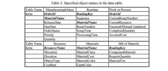
• Define the tables with the specified object name and import data, as shown in Table 2 (the items in bold and italic font are the key column in the model);
• Modify the resource location to the defined position in the facility window (in proportion to Figure 1),
• Modify the Consume time and Produce time to 0, and set the Processing time (as shown in Table 1) for each processing step in the Processing Tasks menu.
• Add the vehicle and path to connect the source (Order Arrives), resources, and sink (Ship) in the facility window;
• Change the transport logic for each node that needs to transfer a workpart via a vehicle.
• Set the simulation time and run the model.

The model can be construct with these main steps and several minor changes. Figure 4 shows a screen shot of the FMS factory model animation. It should be noted that the animation pictures of the machines are not real ones, but are rather representative drawings selected from the symbol library.

The model can be validated and verified through the model animation and numeral tests with the simple order example.

4 APPLICATIONS

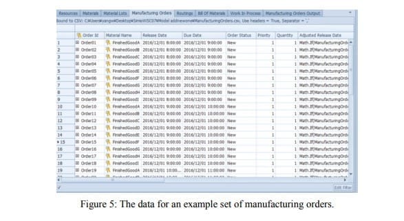
In this section, the scheduling experiments for the cases of a usual state and a new order is implemented. The initial product-mix numerical example uses 2 set (i.e., two pieces) of each product for the experiments. In the initial status, the order release date and the order due date are one hour apart, i.e., in the first working hour, orders arrive for one piece of each product. The due date of the first set orders is one hour after the start of the simulation, at which time the second set of orders for 1 set (i.e., one piece) of each product arrives. The data for an example set of manufacturing orders is shown in Figure 5.

4.1 The Scheduling Results of the Model

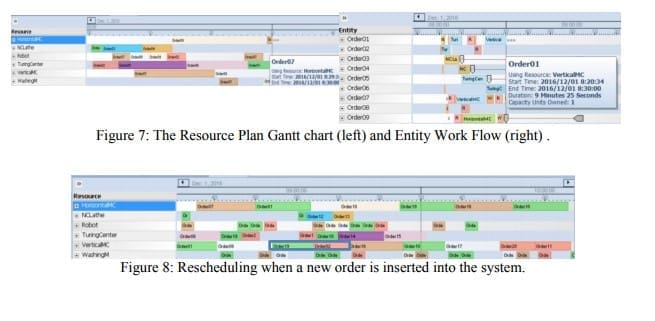
After importing the data table into the model, a schedule can be created in the Planning tab. The generated schedule under the First in First Out rule is shown in Figure 6. The Entity Workflow Gantt chart (Figure 6, right) shows the scheduling of the how jobs seize the resource, as well as the milestones and targets status for each order. In addition, the Resource Plan (Figure 6, left) shows how each resource in the system is utilized by the jobs. Furthermore, the activities of the entities and resources are traced by the usage Logs that display the shop floor at a defined time point. moreover, different resource dispatching approaches can be compared by setting the Ranking Rule and Dynamic Selection Rule under Resources.

4.2 The “Insert the new Orders” Case

In a real usage situation, there is a high probability that the system encounters a new order. If there is one order of product A and one order of product B received 30 minutes after production started (Order Release Time: 8:30; Order Due Time: 9:30). In this case, the Work in Process (WIP) order as well as the degree of progress made in the processing and the completed order can be confirmed through the output table. Furthermore, a VBA program is developed for generate WIP table using for rescheduling. The schedule generated under the Most Work Remaining rule at 8:30 is shown in Figure 7.

By loading the partially completed orders into the WIP table and importing the new orders (Order 19, Order 20) into the Manufacturing Orders table, the model can perform rescheduling. Figure 8 shows the Resource Plan Gantt chart when the system inserts two rush orders. Furthermore, in the processing sequence, Order 02 comes after the new order, Order 19, because of the defined rule for resource dispatching.