A Generic Framework for Modeling Airport Operations at A Macroscopic Level

by Paolo Scala, Miguel Mujica, Daniel Delahaye, Ji Ma

As presented at the 2019 Winter Simulation Conference

Abstract

In this paper, a general approach for modeling airport operations is presented. Airport operations have been extensively studied in the last decades ranging from airspace, airside and landside operations. Due to the nature of the system, simulation techniques have emerged as a powerful approach for dealing with the variability of these operations. However, in most of the studies, the different elements are studied in an individual fashion. The aim of this paper, is to overcome this limitation by presenting a methodological approach where airport operations are modeled together, such as airspace and airside. The contribution of this approach is that the resolution level for the different elements is similar therefore the interface issues between them is minimized. The framework can be used by practitioners for simulating complex systems like airspace-airside operations or multi-airport systems. The framework is illustrated by presenting a case study analyzed by the authors.

Introduction

The air transport system, has the main objective of connecting cities, countries, continents and people from different parts of the world. Air transport system, can be modelled as a network of nodes and links, where the nodes are the airports and the links are the routes connecting them. In this context, the airport can be defined as the infrastructure intended to accommodate the flow of aircraft within the air transport network with the purpose of transporting passengers and/or freight.

In 2017, European air traffic saw a big growth, reaching 10.6 million flights, surpassing the last record of 10.2 million in 2008. Comparing to 2016, in 2017 there were 4.3% of more average daily flights as it is shown in Figure 1. Passenger at European airports in 2017, were 8.5% higher than those in 2016. Figure 2 shows the major airport in Europe in terms of passenger and aircraft movements, with the top five airports having an amount of passengers above 63 million and aircraft movements above 449 thousand, each of them had an increase in both passenger traffic and aircraft movements between 2016 and 2017 (EUROCONTROL 2018).

On the other hand, this constant growth has put pressure on airports, to which for some of them, capacity limit has already been reached. Environmental constraints, societal, technical and land use restrictions On the other hand, this constant growth has put pressure on airports, to which for some of them, capacity limit has already been reached. Environmental constraints, societal, technical and land use restrictions

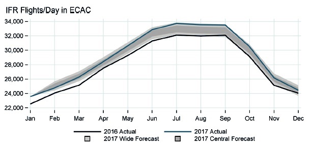
Figure 1: Comparison between air traffic in 2016 and 2017.

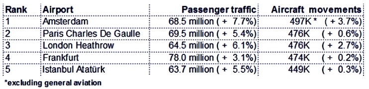
Figure 2: Top five European airports in terms of passenger traffic and aircraft movements in 2017.

In the last decades, studies about airport operations have been focused on improving their efficiency and effectiveness with the aim of improving airport capacity, both for airspace (Kleinman et al. 1998; Zuniga et al. 2013; Zheng et al. 2015; Klein 2017), and ground operations (Khoury et al. 2007; Martinez et al. 2014). These studies implement simulation techniques for evaluating airport performance. This highlights the relevance of using modeling and simulation for dealing with such problems. Moreover, there are various specific-purpose simulation software related to aviation operations on the market, such as AirTop (Transoft Solutions 2018) and CAST (Airport Research Center 2018). These software include different modules for modelling airspace, airside and terminal operations. The use of a DES gives some advantages such as: visualization, time compression and expansion, use of stochastic variables, running experiments with several replications. We can classify simulation software in: specific-purpose and generalpurpose ones. The first ones, use predefined objects with characteristics related to the specific field of interest, while general-purpose ones include some predefined objects that can be used by the developers to create any kind of model for any kind of field of interest. By using general purpose simulation software users and developers are more flexible in developing extended and ad-hoc logic of the system. In this work, a simulation model of airspace and airport ground operations was developed by using a general-purpose simulation software, in this way, a tailored model could be developed.

The aforementioned works focus on specific airport operations, such as airspace and/or ground, and do not consider airport operations in a holistic view. In Scala et al (2017a), a model that considered airport operations with airspace and ground operations together was made. A downside of this work, was that the model could not be used as a general approach since different abstraction levels were used for approaching a particular problem.

In this paper, in order to overcome this limitation, a macroscopic level approach of airport operations is proposed. This approach, allows to build a general framework where airport operations can be modeled, regardless of the size and the layout by just using general elements from queue and network theory. The advantage of making it a general one, is that it is suitable for a smooth coupling of optimization algorithms that are able to consider most of the elements of the whole system using a holistic approach, thus making it suitable for studying complex systems like airspace-airside or multi-airport systems. This framework, has been used successfully for implementing different techniques like optimization (Ma et al. 2019) and also the integration of the simulation and optimization (Scala et al. 2017b; Scala et al, 2018), but it has never been formalized. To test the validity of the framework, it has been applied to a real case study by means of a simulation model.

The main contributions of this paper are threefold: first, the development of a canonical framework for modeling airport operations in a general fashion, thus enabling the modelling of different elements like airspace and airside operations together; second, it formalizes a framework where different techniques can be implemented, such as optimization and/or simulation; third, it provides a guideline for enabling analysts to model airport operations in a systematic way.

The remaining of the paper is as follows: in section 2 the generic framework for modeling airport operations is presented, in section 3 the approach is applied to a real case, and a simulation model is presented. In section 4 conclusions are drawn.

Airport Operations at a Macroscopic Level

In this section, a generic framework for modeling airport operations is presented. The airport operations are modeled at a macroscopic level, in this context, macroscopic approach refers to the level of detail of the different components of the final model. The airport airside components considered were: runways, taxiway network and terminals; these components were modeled as resources characterized by a maximum capacity and an occupancy time. Airspace operations, on the other hand, were the ones related to the approaching routes toward the airport, such as aircraft sequence, and merging to the final approach route before landing to the runway. Airspace operations were modeled in more detail, modeling airspace performance flight-byflight.

This framework, allows to consider these operations together or separately, depending on the type of analysis we want to conduct. For example, a multi-airport system can be modeled by aggregating the airside components of each airport of the system and by including the airspace component as a common component for the airports. Furthermore, different techniques such as optimization can be coupled to one or more components, or to the whole airport system. Figure 3, provides a representation of how a multi-airport can be developed, and how optimization process can be included in the framework proposed in this work. In Scala et al. (2017, 2018), this framework was successfully applied using an optimization algorithm for optimizing the whole system performance and evaluating this the solution by means of a discrete event simulation model, in this way, a feedback loop could be created for enhancing the system performance.

In the following sections, the modeling of airspace and airside operations are described in more detail.

Airspace Modeling

The airspace surrounding airports, commonly called terminal maneuvering area (TMA), is a portion of airspace where aircraft fly their approaching and departing routes. Especially for busy airports, it can be a congested area due to the traffic converging to the runways and also due to the outbound traffic. When the aircraft fly under instrument flight rules (IFR), their flight path is facilitated by the implementation of Standard Arrival Routes (STARs) and Standard Instrument Departure Routes (SIDs). STARs and SIDs are standard routes that expedite the safe and efficient flow of air traffic operating to and from the same or different runways. STARs and SIDs are published routes that can be followed by the flight crew unless the air traffic controllers give different instructions.

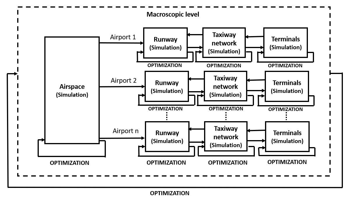
Figure 3: Modular framework for implementing simulation and optimization techniques.

Each runway can have one or more STAR/SID, each of them ensures aircraft to fly at a certain altitude level, under speed restrictions and following some significant points (waypoints). The last descending path before landing, under IFR, it is called instrument approach procedure. This procedure includes a series of predefined maneuvers that leads to landing at a predefined runway. The instrument approach procedure can be divided in two main segments, named initial approach segment and final approach segment. In some cases, another additional segment can be part of the instrument approach procedure, the intermediate approach segment. Figure 4 shows a schematic representation of them.

Figure 4: Schematic representation of the landing routes (STAR and instrument approach procedure).

The operations carried out in the TMA, under IFR, are restricted by predefined constraints that involve speed, and separation between consecutive aircraft. Speed limits can be consulted in the STARs and SIDs routes that are published by the air traffic service (ATS). In this context, speeds refer to calibrated air speed (CAS), as it may differs from ground speed (GS). Usually, an aircraft entering the TMA from one of the STARs, it is not allowed to fly at a speed that exceeds 250 kts. Other specific speed limitations can be found in other significant waypoints along the STAR, and in the main waypoints of the instrumental approach procedure such as IAF, intermediate fix (IF) and final approach fix (FAF). During the flight, aircraft progressively slow down until they reach the FAF waypoint, where the final descending speed is reached and kept until touching down to the runway. The same concept is applied to the SIDs, where aircraft fly at a certain speed based on the speed limits defined on each waypoint placed along each SID. Concerning the separation minima, there are two different separations that must be respected due to safety reasons: horizontal and vertical. Horizontal separations are ensured in terms of longitudinal and lateral separation. Longitudinal separation minima between two consecutive aircraft depends on the aircraft type of the leading and trailing aircraft, in this context the International Civil Aviation Organization (ICAO) (ICAO 2016) has defined the different separation minima. The lateral separation between two consecutive aircraft is ensured by referencing to different geographic locations and/or by referencing to the same navigation aid. Vertical separation is ensured by leaving at least 1000 ft (300m) of vertical distance between two aircraft.

The airspace landing routes (STARs), were modelled as a network of links and nodes. Each node represented a waypoint of the route, and the link the connections between waypoints. In each node, logic such as speed-check and separation minima-check were implemented. On each link, properties such as link length, maximum capacity on the link, and maximum speed on the link could be set. By setting these properties and logic on each node and link of the airspace network, it is possible to create a general framework for modeling different airspace. When modeling any other different airspace, the nodes and links will keep the same properties, while the only difference will be the layout of the network.

Airport Airside Modeling

The chronological order of the operations performed on the airside is the following: the aircraft lands on the runway, crosses the taxiway network and then parks at the terminal. After the turnaround time, the aircraft crosses again the taxiway network in order to reach the departing runway. The airside components such as runway, taxiway network and terminals, are modeled using elements which related to queueing theory, like the server element. A server element, can process a maximum number of entities simultaneously and processes each entity according to a specific processing time. Queueing theory analogy fits well with the way airside operations were modeled at the macroscopic level, in fact, runways, taxiways and terminals can be seen as servers with a maximum capacity and a specific processing time, and aircraft can be seen as the entities to be processed. In this framework, runway, taxiway network and terminal components are logically connected by following the chronological order of the operations. This way of modeling gives the user high flexibility for modeling different airport layout, since both capacity and service time values can be changed according to the specific airport characteristics. Airside performance are evaluated on each component in terms of their utilization. The main properties of the runway component are: capacity, which is set to one, since only one aircraft can use the runway at a time; and runway occupancy time. The main properties of the taxiway network component are: maximum capacity of the taxiway network, which is the maximum number of aircraft that can cross simultaneously the taxiway; and taxiway occupancy time. The main properties of the terminal component are: maximum capacity, which is the number of gates of the terminal; and the turnaround time, which is the time that starts when an aircraft parks at a terminal gate and ends when it leaves the terminal gate.

In Figure 5, a schematic representation of the macroscopic approach for a single airport is depicted. As it can be seen from the example of Figure 5, the airspace network is connected with two landing runways, which in turn, are connected with the taxiway network component. The taxiway network, connects both terminals and departing runways.

Inputs and Outputs of the Model

The inputs of the model are given by the flight schedule and by the initial parameters of the system. The flight schedule contains all the information needed by the entities (aircraft) such as: flight type, aircraft size, terminal number, entry point in the airspace, entry time in the airspace, entry speed in the airspace, landing runway, pushback time, and departing runway. The initial parameters of the system, are static parameters to be set before running the model such as: terminal capacity; taxiway network capacity; landing speed; average taxi time; runway occupancy time.

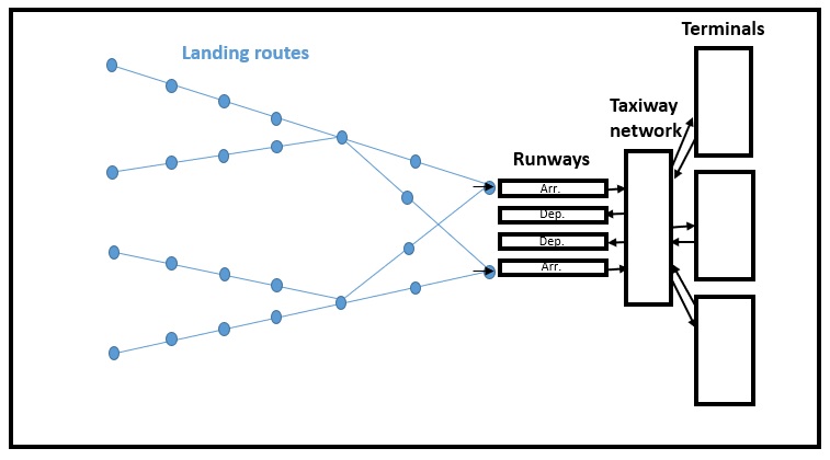
Figure 5: Schematic representation of the airport operations at a macroscopic level.

The output of the model is related to the evaluation of the system performance in terms of congestion. The outputs used are: congestion level in the airspace and congestion level on the airside. The first is calculated as number of aircraft conflicts in the airspace, where conflicts are defined as any violation of longitudinal separation minima between consecutive aircraft. The longitudinal separation minima are standard values provided by ICAO (ICAO 2016).

General Assumptions

The assumptions of the model are related to:

• Aircraft acceleration in the airspace is considered constant, and it is calculated based on the entry speed in the airspace, the landing speed and the descending route length
• Runway and taxiway occupancy time are modeled as average values
• Aircraft can park at any gate of the assigned terminal
• Terminals are modeled as virtual nodes, and their capacity is given by the number of gates available
• The taxiway network is modeled as a virtual node with a certain capacity
• The landing speed is a constant value based on the aircraft size (heavy, medium, small)
• Aircraft in the airspace are considered to be enough vertically separated
• Departing routes in the airspace are not considered
• The effect of the wind is not considered

Case Of: Paris Charles de Gaulle Airport

In this section a discrete event simulation model representing the airport operations at a macroscopic level is presented. The model is based on a real case study, which is, Paris Charles de Gaulle airport (PCDG). The simulation model was developed by using a general-purpose simulation software, SIMIO (SIMIO 2019), however, by using the framework proposed any general-purpose simulation software or any programming language can be used to develop the models. In this paper we will refer to it as “Simulation Model”. In the description are mentioned some of the most common objects that can be found in any general-purpose simulation software. Furthermore, the simulation model has been validated using the Historical data validation approach (Sargent 2007), as it represents a critical aspect in the development of any simulation model.

Model Development

In Figure 6 a schema of the simulation model is given, by including the main objects utilized for building the model.

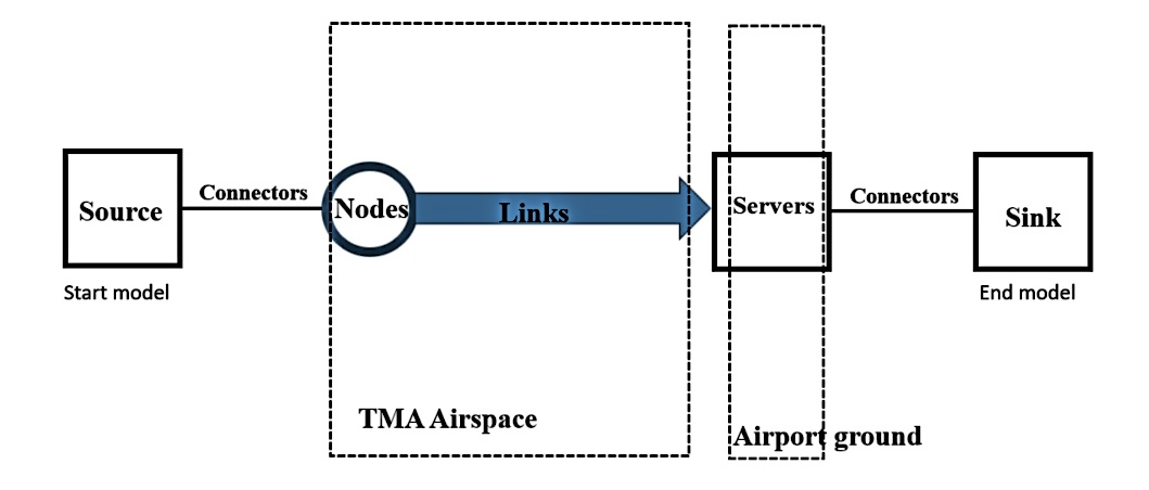
Figure 6: Schema of the simulation model.

The airport TMA airspace was modelled as a network of node objects and path objects, representing the waypoints and segments of the landing routes. In each node, logic such as speed-check and separation minima-check were implemented. Segments were modelled by using paths, where properties such as length, maximum capacity, and maximum speed could be set. Figure 7 shows the animation of the simulation model for the TMA airspace in west configuration of PCDG airport.

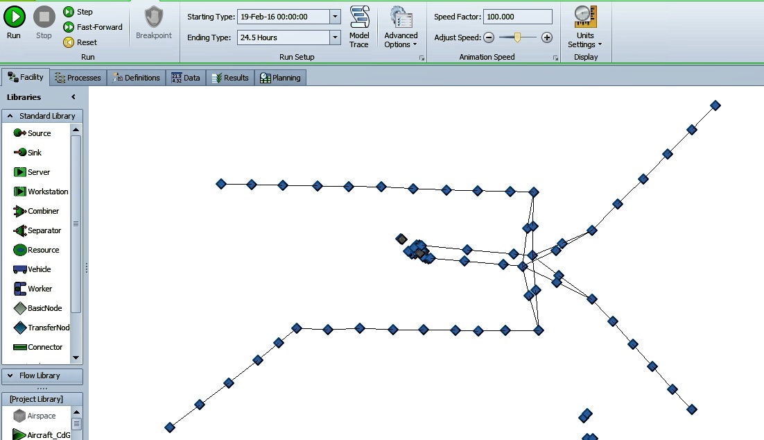
Figure 7: TMA airspace network animation.

In the following list, each model object is described with its main characteristics and functionalities.

• Model paths. Paths represent the segment of the airspace landing routes. The main properties of this object are: the length of the segment; the path type, which can be unidirectional or bidirectional; and the path speed limit, which determines the maximum speed that can be reached on the path
• Model nodes. Nodes represent the waypoints of the airspace landing routes. In the property section it is possible to call some functions called “processes” in order to implement different logic such as separation minima between aircraft and speed updates

Regarding the airport airside components, runways, taxiway network and terminals were modelled by using server objects. Server objects were linked to each other by using connectors, a specific time-zero object path. In Figure 8. it can be seen part of the model animation of the airport airside and how these objects were connected to each other.

In the following list, each model object is described with its main characteristics and functionalities.

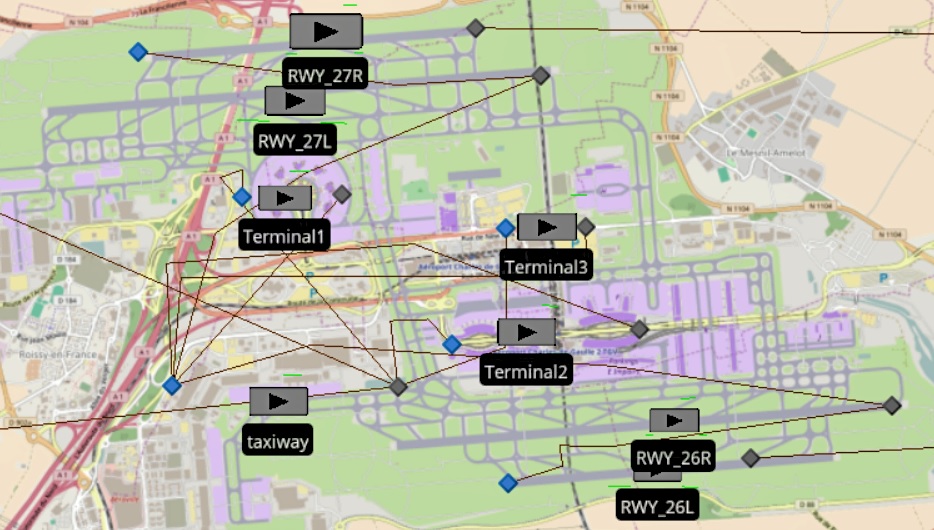
Figure 8: Model elements over the GIS of PCDG.

• Model servers. Server objects were used for modeling airside components such as runways, taxiway network and terminals. The main properties of this object are: capacity, which sets the maximum number of entities that can be processes by this object simultaneously; and processing time, which sets the amount of time that each entity will be processed by this object
• Model source. The source object is used for creating the entities of the model. The source generates entities according to a flight schedule. The main properties of this object are: the entity type, which define the entity to be created; and the arrival mode, which is the way the entities are created, following an interarrival time, a specific schedule and so on
• Model sink. The sink object is placed at the end of the model and it is used for destroying the entities. Usually in the sink object there are no many properties to be set, however, in this object, it is possible to call “processes” for modeling specific logic

Implementing the logic of the model in SIMIO is possible with the use of the process feature. A process is a logical sequence of steps (see Figure 9). Once a process is created, it can be called by different objects within the model. Each step allows to do a specific action. The main steps used in the model are: Assign, Decide, Delay, Wait, Fire, Execute and SetNode.

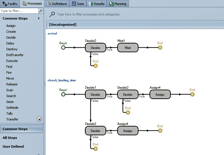
Figure 9: Processes in SIMIO.

In the following list, they are described:

• Assign: assigns a value to a variable
• Decide: based on a condition or a probability, the entity can exit a true or a false exit, in this way if-then-else statement can be implemented
• Delay: delays the occurrence of an event
• Wait: allows an entity to wait until a specific event is triggered (“fired”)
• Fire: triggers (“fires”) an “Event”
• Execute: executes a “Process” within another “Process”
• Set Node: sets the node destination to an entity

Validation of the Model

In order to validate the simulation model, the authors chose to apply the validation method: Historical data validation (Sargent 2007). This method is implemented when historical data is available. The method consists in using part of the data for building the model and using part of the data for validating it. In this work, the data used for building the model refers to the number and capacity of each components of the system such as: airspace approaching routes, runway and taxiway system and terminals. Average runway occupancy time as well as average taxiway and terminal occupancy time were derived from the historical data available. In Table 1, the main components of the airport are listed, for each of them, significant information about capacity is given.

Table1: Main airport system components (PCDG).

The average runway occupancy time, for both landings and take offs, was assumed as 60 seconds. The taxiway occupancy time was assumed as an average derived from historical data. Taxiway occupancy time depend on the specific couple runway-terminal, these values are shown in Table 2.

Table 2: Average values of taxiway occupancy time (seconds).

The historical data used for the validation of the models is the flight track taken from the radar, for one day of operations. In this data each aircraft is tracked in the airspace and in the airside, therefore, entry time in the airspace, landing time, entry and exit time to/from terminals and take off time are collected. The statistic test used for the validation is the standardized mean difference (SMD), this test is part of the effect size statistic framework. The effect size is used for quantifying the degree of the deviation between two samples (Vacha and Thompson 2004). This test is preferred when compared to the t-test, due to the size of the samples. As using the t-test for a big data sample, would consider any small difference as significant. The variables used in order to implement the validation are the occupancy over time of the runway, taxiway and terminals. In the SMD we calculate the value 𝛿 which represents the magnitude of the deviation between the output from the historical data and from the simulation model. The value of 𝛿, is given by equation 1,

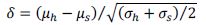
where, 𝜇&is the average value of the historical data observations for each variable; 𝜇( is the average value of the simulation model output for each variable; 𝜎& is the standard deviation of the historical data for each variable; and 𝜎( is the standard deviation of the simulation model for each variable. A value of 𝛿 close to zero, means that the simulation model accurately represents the real system output. In tables 3, the statistics about the historical data and simulation model, for each variable, are shown. In Table 4, the value of 𝛿 for the SMD analysis is shown.

By looking at the results of Table 3, we can notice that regarding the runway occupancy, in the simulation model, runways appear to be more loaded as the average values are higher, as well as the standard deviations. Regarding the taxiway network occupancy, simulation model shows a less load on the taxiway compared to the original data, as average and standard deviation values suggest. Regarding the terminals, there is very little difference between the original data and simulation model average and standard deviation.

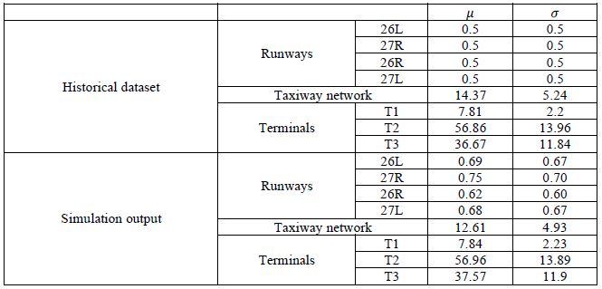
Table 3: Statistical analysis for each variable.

Looking at the values of 𝛿 for each variable analyzed in Table 4, we can derive that the magnitude of the deviation between the two datasets, historical and simulated, is not significant. The highest value of 𝛿 can be found for the taxiway network, which is 0.34, however, this value is close to zero. The variables regarding the runways, have values that range between -0.22 and -0.32, also for these variables the 𝛿 values are close to zero, which is the ideal scenario. The smallest value of 𝛿 is found for the terminals, with values that range between -0.01 and -0.007, revealing that the simulation output reproduces well terminal performance of the real system. Overall, the SMD test has highlighted that the simulation mode reproduces accurately the real system.

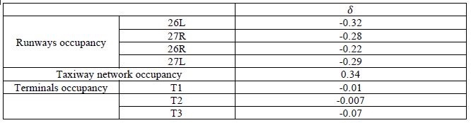
Table 4: SMD analysis for each variable.

Conclusion

This paper presents a generic framework for modeling airport operations. This study serves as a guidelines for modeling and simulating similar systems. Due to the standard characteristics of the model, it can be adapted to any (multi)airport system, regardless of the size and layout. Furthermore, the different components of the framework, such as airspace and airside, can be used to conduct aggregate or separate analyses. The framework presented is also suitable to incorporate different techniques such as simulation and optimization, as it was shown by applying it to a real case study by means of a simulation model. The simulation model was developed by using a general-purpose simulation software. In the paper, the authors provided a description of the objects used for modeling the operations, so that the model can be reproduced by any other commercial general-purpose simulation software. The simulation model, was validated by using a statistical approach, proving to be able to model the airport operations accurately, reinforcing the validity of the framework.

Acknowledgments

The authors would like to thank the AUAS-AMSIB and -Aviation Academy for supporting this study, as well as the Dutch Benelux Simulation Society (www.DutchBSS.org) and EUROSIM for disseminating the results of this work.

Author Biographies

PAOLO SCALA is a PhD student at l’Ecole Nationale de l’Aviation Civile (ENAC) (France) sponsored by the Aviation Academy and the Amsterdam School of Internatrional Business (AMSIB) of the Amsterdam University of Applied Sciences (AUAS) (the Netherlands). His research interests lie in modeling and simulation and optimization applied to the aviation field. His email address is p.m.scala@hva.nl.

MIGUEL MUJICA is an Associate Professor at the Aviation Academy of the Amsterdam University of Applied Sciences (AUAS) in the Netherlands. His research interests lie in simulation techniques and O.R. in industrial, logistics and aviation problems. His email address is m.mujica.mota@hva.nl.

DANIEL DELAHAYE is a Professor at l’Ecole Nationale de l’Aviation Civile (ENAC) (France). His research interests lie in stochastic optimization for airspace design and large-scale traffic assignment. His email address is delahaye@recherhe.enac.fr.

JI MA is a PhD student at l’Ecole Nationale de l’Aviation Civile (ENAC) (France). Her research interests lie in the airport traffic optimization. Her email address is ji.ma@recherche.enac.fr.